It’s hard to overestimate the importance of modeling tail risk when it comes to the care and feeding of investment portfolios. But where to begin? The topic of studying, estimating and otherwise dissecting rare but extreme market events can be a black hole of analytical possibilities and econometric complexity. It’s also too important to be left as a plaything for rocket scientists. With that in mind, here begins the first in a series of statistical investigations into the realm of return distributions when the tail wags the dog.

The vehicle for navigating the numbers on our exploratory journey is R, a powerful tool for studying the cryptic corners of tail risk. If you’d like to replicate the results below, you can find the code here.

Let’s begin this primer with a simple observation: ours is a fat-tailed world. Measuring the associated risk, alas, is devilishly difficult, at least in terms of developing a high level of confidence that you’ve roped and wrangled the beast to any great degree. But while definitive modeling of future events is destined to leave plenty of room for uncertainty, we can and should make an effort to wrap our heads around the outer edges of market risk. Why? Because stress testing portfolio strategies may reveal design flaws. In that case, it’s best to consider the cracks in the foundation within the comfort zone of modeling possible scenarios. Surprises in real time with real money, by contrast, are to be avoided whenever possible.

This much is clear: most portfolios are vulnerable in some degree to tail risk. Exactly how vulnerable is difficult to estimate with any certainty, although we can at least chip away at the haze through the process of modeling these events.

Let’s start by recognizing the foundation of tail-risk analysis: market returns aren’t normally distributed, at least not all of the time. Although a bell-shaped curve with thin tails—predictably low extreme returns—is a reasonable approximation of market action over long sweeps of history, extreme losses occur with greater frequency than you would expect in a normal distribution.

The most popular measure of estimating the probability of loss in the extreme is value-at-risk (VaR).  Although this metric has well-known defects, it’s still widely used in the financial industry. Why? Jon Danielsson explains in Financial Risk Forecasting that “when one considers its theoretical properties, issues in implementation and ease of backtesting, the reason becomes clear. VaR provides the best balance among the available risk measures and therefore underpins most practical risk models.”

Minds may differ on that point, but VaR is one possibility as a starting point. It doesn’t hurt that we can easily estimate VaR with a few lines of code. First, define the confidence levels—let’s use the standard 95% and 99% (using the reciprocals in this case) and then generate the associated quantiles. For instance, assuming a normal distribution, VaR is calculated as:

[code language=”r”]
p <- c(0.05,0.01) # reciprocals of 95% and 99% confidence levels
VaR.1 <-qnorm(p)
[/code]

As a simple modeling example, let’s assume a portfolio with a normally distributed expected mean return of 7% and a standard deviation of 15%. The associated VaR for a $100 portfolio is $17.67 at the 95% confidence level and $27.89 at the 99% level, calculated with the quantile function:

[code language=”r”]
alpha <- c(0.95, 0.99)
VaR.sim.1 <-qnorm(alpha,mean=-0.07,sd=0.15)*100
[/code]

VaR tells us the best-case scenario for tail risk. In other words, this is the estimate for the minimum worst-case loss. But a more realistic modeling effort should consider what lies beyond that best-case estimate. For that calculation, we can call what’s known as estimated shortfall (ES), which is also referred to as conditional VaR (CVaR) or expected tail loss (ETL). Crunching the numbers for ES is a simple extension of the VaR formula via the distribution function:

[code language=”r”]
dnorm(qnorm(p))/p
[/code]

The equivalent ES estimate (via Dr. Nikolay Robinzonov) for a $100 portfolio with a normally distributed expected mean return of 7% and a standard deviation of 15%:

[code language=”r”]
alpha <- c(0.95, 0.99)
ES.sim.1 <-(-0.07 + 0.15 * dnorm(qnorm(alpha))/(1 – alpha))*100
[/code]

The resulting ES is $23.94 (95%) and $32.98 (99%). Not surprisingly, the estimated ES loss is greater than the VaR projection because we’re looking at risk beyond the stated confidence levels.

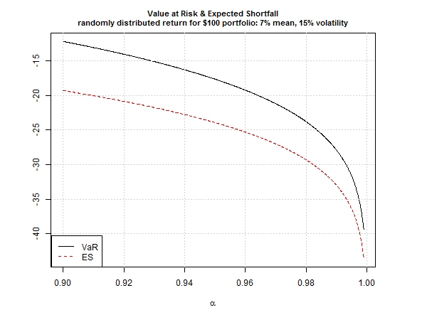
For perspective, consider how various risk assumptions compare across several confidence levels, ranging from 90% up to 99.9%.

Note that the ES (red line) reflects larger losses vs. VaR at all the confidence levels. Because tail losses, when they occur, are likely to exceed VaR’s projection, ES is a more practical estimate of what’s lurking in extreme market events.

But there’s a problem: we’re assuming a normal distribution. For a more realistic estimate, it’s prudent to anticipate that we’ll encounter fat tails at some point in our investment travels. Let’s factor this into our ES estimate for this test portfolio using the Student’s t-distribution (with code below again courtesy of Dr. Robinzonov). Unsurprisingly, the adjustment boosts ES. For example, the expected loss on our $100 portfolio for ES at the 95% confidence level is $26.52 vs. $23.94 for ES based on a normal distribution.

[code language=”r”]
alpha <- c(0.95, 0.99)
mu=0.07
nu=5 # degrees of freedom
lambda <- 0.116 # scaling parameter which approximates 0.15 volatility
nu=5 # degrees of freedom
ES.sim.students.1 <-(-mu+lambda*dt(qt(alpha, df=nu),df=nu)/
(1-alpha)*(nu + qt(alpha,df=nu)^2)/(5-1) )*100
[/code]

This is merely the tip of the iceberg in the search for greater realism in modeling tail risk. For example, we might also consider what’s known as modified VaR (M-VaR) and ES (M-ES) applications, which factor in non-normal (skewed and/or kurtotic) distribution assumptions. Fortunately, R makes it easy to calculate these alternative risk metrics via the PerformanceAnalytics package.

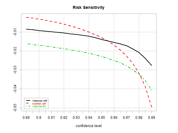
As one demonstration based on a globally diversified portfolio (see definition below), here’s how standard VaR based on daily historical data (12.31.2000 through 7.10.2015) compares with M-VaR and the historical estimate of ES via the chart.VaRSensitivity function. Note that at the higher confidence levels, M-VaR (red line in chart below) exceeds the projected loss of the standard ES (green line).

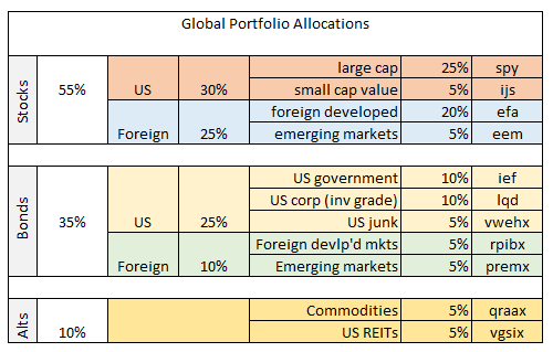
Finally, let’s crunch some numbers using ETF data for a globally diversified portfolio as follows:

If this was a real portfolio we’d review tail risk from multiple dimensions. For now, let’s compare a rolling 12-month estimate of M-ES vs. monthly returns for a buy-and-hold version of the strategy from 2003 through June 2015 via the chart.BarVaR function in the PerformanceAnalytics package. This is a toy example, but it’s a reminder that M-ES—and all risk metrics, for that matter—aren’t static. The time window you select, along with the choice of risk metric, will deliver different results, perhaps dramatically so. As such, it’s essential to develop risk estimates carefully, which will depend on a number variables, including risk tolerance, investment horizon, goals, etc.

In future posts, I’ll consider how to enhance this preliminary look at tail risk. There are several possibilities, including forecasting and developing a richer set of historical estimates. It’s safe to say that we can improve upon the basic applications outlined above. The future’s still uncertain, of course, and no amount of sophistication in modeling can change that simple fact. That said, we can still add value over risk expectations based on naïve assumptions or even the foundational concepts discussed so far. How much value? The answer depends on what you’re expecting. Regardless, it’s best to keep expectations under control. But if your assumptions are reasonable, modeling tail risk can be a productive exercise. That may not be obvious until we dive deeper into the numbers. Stay tuned….