Managing risk via tactical asset allocation (TAA) offers a number of encouraging paths for limiting the hefty drawdowns that take a toll on buy-and-hold strategies. But what looks good on paper can get ugly in the real world. There’s a relatively easy fix, of course: consider the total number of trades associated with a strategy as another dimension of risk.
The dirty little secret is that many TAA backtests don’t survive the smell test after considering the impact of trading frictions—particularly for taxable accounts. Deciding where to draw the line for separating the practical from the ridiculous varies, based on the usual lineup of factors—an investor’s risk tolerance, time horizon, tax bracket, etc. But there’s an obvious place to start the analysis. Let’s kick the tires for some perspective using some toy examples.
An obvious way to begin is by using the widely cited TAA model outlined by Meb Faber in what’s become an staple in the literature for this corner of finance—“A Quantitative Approach to Tactical Asset Allocation”. The original 2007 paper studied the results of applying a simple system of moving averages across asset classes. The impressive results are generated by a model that compares the current end-of-month price to a 10-month average. If the end-of-month price is above the 10-month average, buy or continue to hold the asset. Otherwise, sell or hold cash for the asset’s share of the portfolio. The result? A remarkably strong return for the Faber TAA model over decades, in both absolute and risk-adjusted terms, vs. buying and holding the same mix of assets.
The question is whether running the Faber model as presented would be practical after deducting trading costs and any taxable consequences? Let’s ask the same question for two other simple strategies:
Percentile strategy: apply the rules in Faber but limit the buy/hold signal so that it only applies when the asset price is above the 70th percentile for the ratio of the price above the trailing 10-month average. The same logic applies in reverse for the sell signal: the asset price is below the 30th percentile for the ratio of price below the 10-month moving average. For signals between that 30th-70th percentile range, the previous signal remains in force.
Relative-strength strategy: apply the Faber rules but limit the buys to assets in the top half of the performance results for the target securities, based on the trailing 10-month results. The same rule applies in reverse for triggering a sell signal. In other words, sell only assets in the bottom half of the performance results via the trailing 10-month period if a sell signal applies.
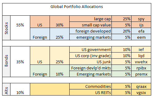
Note that for all strategies the signals are lagged by one month to avoid look-ahead bias. To test the strategies we’ll use the following portfolio (see table below), which consists of 11 funds representing a global mix of assets, spanning US and foreign stocks, bonds, REITs and commodities. In essence, this is a global twist on the standard 60%/40% US stock/bond mix. The initial investment date is the close of 2004 with results running through this month as of Feb. 26. All the models start with the same allocation.
The chart below compares the results for the three strategies and a buy-and-hold portfolio. The Faber model delivers the best results. A $1 investment in the strategy at 2004’s close was worth roughly $1.48 as of last Friday. The Relative Strength model was in second place at $1.39, followed by the Percentile Strategy ($1.34) and Buy and Hold ($1.20). Raw performance data tells us that the Faber model is the winner.

Note, too, that all three TAA models deliver superior results in risk-adjusted terms. For instance, historical drawdown for the three strategies is relatively light compared with the Buy and Hold model. In particular, the Buy and Hold portfolio suffers a hefty drawdown in excess of 40% in 2008-2009 whereas the three TAA models never venture below a roughly 10% drawdown.

Given what we know so far, it appears that the Faber model is the superior strategy via a mix of strong performance and limited drawdown risk. But the results look quite a bit different once we add in the dimension of total trades associated with each strategy. Buy and Hold, of course, excels on this front. But the lack of trades (or trading costs) is more than offset by the steep drawdown for Buy and Hold.
The question, then, is what is the superior TAA model if we consider real-world costs? The numbers provide the answer via a summary of total trades for each strategy, as shown in the table below. The Percentile model’s trades number just 93 for the 2004-2016 test period—less than half the trades for other two strategies. The Percentile model’s total return trails the Faber results, but only modestly so. In short, the Percentile model generates 90% of the Faber model’s returns, with a comparable level of superior drawdown risk compared with Buy and Hold. Add in the Percentile’s substantially lower turnover clinches the deal, or so one could argue.

If this was an actual consulting project we would run additional tests before making a final decision. For instance, we might consider other models and look at longer historical periods, perhaps using daily prices and compare results with a variety of risk metrics. Running Monte Carlo simulations to effectively test the models thousands of times would be useful too.
Looking at the results in terms of the number of trades associated with each strategy is no less valuable. This subtle but crucial aspect of backtesting tends to be ignored. But if you’re comparing TAA models for use in the real world, it’s essential to adjust for real-world trading frictions. In some cases, adding this extra layer of analysis may end up as a determining factor for separating failure from success.
* * *
Previous articles in this series:
Portfolio Analysis in R: Part I | A 60/40 US Stock/Bond Portfolio
Portfolio Analysis in R: Part II | Analyzing A 60/40 Strategy
Portfolio Analysis in R: Part III | Adding A Global Strategy
Portfolio Analysis in R: Part IV | Enhancing A Global Strategy
Portfolio Analysis in R: Part V | Risk Analysis Via Factors
Portfolio Analysis in R: Part VI | Risk-Contribution Analysis
Tail-Risk Analysis In R: Part I
Managing Portfolio Risk With Tactical Asset Allocation
Can you provide a link with a fuller explanation of the percentile strategy?
Tony,
The percentile strategy is the Faber strategy with a filter. For the standard Faber rules: any time the current price is above (below) the 10-mo avg in any degree there’s a buy (sell) signal. The percentile strategy simply requires a higher standard: the current price is above (below) the 10-mo avg by more than the 70th percentile (less than 30th percentile). Percentiles in this example are calculated based on the historical return data starting at 12/31/2004.
–JP
Thanks James. I think I understand the concept, but am still not clear on how to calculate the percentile score. 70th (or 30th) percentile of what exactly? Price over a specified period? Could you give an exemplary calculation and maybe what tool you are using to either find that data or make that calculation on an automated basis?
Tony, as a simple example: think of a set of numbers 1 through 10. The 50th percentile would be 5.5, ie, in the middle of the range. In the modeling example I’m calculating the percentile of the ratio, which is the current price/10mo average. For simplicity in this example I’m using the entire historical period of the ratio (2004-2016) to calculate percentile. The analysis is done in R via the pnorm(scale()) function. A roughly equivalent function in Excel can be found in the percentile() function.
–JP
I appreciate your time in responding. I think I get it. The buy signal is only triggered if the current price (on the measurement day) is (1) greater than the 10mo MA, AND (2) the C/MA (current price/current 10mo MA) is >= 70th percentile of all historical (or some relatively long period) C/MA. The intent is to make the signal less sensitive to short term changes and avoid whipsaw around the MA which has significant tax consequences in a taxable account.
But, I am wondering why would one choose the percentile approach over, for example, using a longer term moving average with the basic Faber model?
I am attempting to implement a version of the GTAA13 AGG6 portfolio in a taxable account, which is a relative strength strategy. I’ve made a number of modifications to suit my own circumstances, but one general change intended to avoid some of the momentum based whipsaw is to reduce the number of asset classes to 9 by consolidating a few of the highly correlated asset classes and staying invested in 6, subject to the MA test. I am very interested in optimizing the absolute momentum signal for this taxable portflio as well.
If you are using the entire historical period to calculate percentile, your method suffers from look-ahead bias.
John,
Agreed. If this was a real model it would be necessary to calculate percentile on a rolling-window basis, perhaps by expanding the length of the window through time. The results do, however, reflect a 1-mo lag re: the signals. In any case, the focus here is simply to highlight how different strategies are associated with varying amounts of turnover/trading costs.
–JP
Tony,
You raise a number of good questions, but a robust answer goes well beyond what’s practical to address in comments. That said, a few quick points. First, the toy model outlined here shouldn’t be considered as optimal. Deciding what works best for a real model requires deeper testing. Rather, the point of this exercise was simply to illustrate, somewhat superficially, that similar TAA models can generate dramatically different results on an after-tax/trading-cost basis.
–JP
What is the CAGR , sharpe and drawdown for the strategies?
Pingback: Quantocracy's Daily Wrap for 02/29/2016 | Quantocracy
James,
Do you use price alone or the P/E to determine your percentiles?
MSD,
The percentile is based on the ratio of current price/10-mo avg.
–JP
Keynes,
The drawdowns for the strategies are already available in the chart–second chart labeled “Drawdown History.” Don’t have the CAGR and SR data handy, but I’ll try to update these numbers at some point.
–Jp
Two thoughts come to mind:
> How does the number of significant draw downs impact these numbers. 12 years is hardly an investing lifetime. I’m wondering how things pan out in 30-40 years, with multiple draw downs.
> What is it that makes the Meb process ‘seem’ so much more sensible; fewer huge drawn downs for instance. However in the end despite not dropping 40% in one fell swoop the difference overall doesn’t reflect this. What element of the philosophy in the end stunts the returns?
> OK, three if I retired in the summer of 2007 I bet I’d know which approach I was taking.
Thanks for the great review of 3 interesting approaches.