The dark art/science of modeling the future has a shady reputation generally, and rightly so. But while extreme caution is always recommended when trafficking in prognostication, it’s a necessary evil to some extent. But some versions of this sorcery are a lesser evil than others. The best of the bunch is arguably combination forecasting, as decades of research advise. Let’s test the recommendation and see if the results hold up.

An early rationale for aggregating individual predictions as a tool for improving the success rate of forecasts goes back nearly half a century to “The Combination of Forecasts,” by J.M. Bates and C.W.J. Granger, Operational Research Quarterly, 1969). Countless studies have followed. Let’s add one more, albeit with a simple test of predicting the near-term trend for the labor market.

Let’s keep things simple and focus on a one-step-ahead forecast for rolling 1-year percentage change for private payrolls using a recursive (expanding window) model, based on the USPRIV data set published by the St. Louis Fed using R to run the analytics (you can find the code here). The test is whether we can improve on a “naïve” forecast, defined here as simply taking the last actual data point and using that as a forecast. If the literature is reliable, we should be able to generate superior forecasts compared with naïve predictions. In fact, that’s what the test below shows.

Before we look at the details, let’s define the individual forecast methodologies that will be combined for the test:

• Vector auto regression (var)
• Autoregressive integrated moving average (aa)
• Linear regression (lr)
• Neural network (nn)

Note that the var and linear regression models are multivariate frameworks—in this case I’m using payrolls in concert with industrial production, personal income, and personal consumption expenditures to generate forecasts. The other two models are univariate, i.e., using payrolls alone for computing predictions. Keep in mind, too, that for this test the selected parameters for each model are more or less default choices, which implies that a superior set-up is possible. But that’s a task for another day.

Meantime, it’s fair to say that each of these forecasting models has a particular set of pros and cons. The question is whether an equally weighted combination of all four is superior to any one model? As we’ll see, the results look encouraging if not necessarily definitive.

For this toy example, the procedure is to train the models based on the rolling one-year percentage changes for private payrolls for the period April 2002 through March 2008. The out-of-sample forecasts begin in April 2008 and run through August 2012. Why those particular dates? No reason—more or less an arbitrary choice.

One quick housekeeping note. The gold standard for this type of test is using vintage data (the initially published numbers before revisions). But such a data set takes some time to build; for simplicity, I’ll use revised numbers. The results will be similar if not exact.

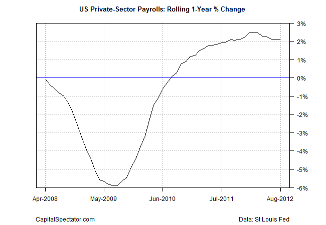
Ok, let’s dive into the details, starting with a recap of the actual results for private payrolls for the time period that we’re trying to forecast.

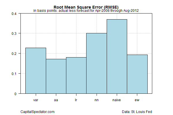
After running the numbers in R, the results are analyzed with a technique known as root mean square error (RMSE) to measure the accuracy of the forecasts. A perfect forecast would have an RMSE value of zero—i.e., zero error. Not surprisingly, all the models have errors, but in varying degrees. The chart below shows that the naïve forecast suffers the biggest error for the sample period, as indicated by the highest RMSE value. The autoregressive integrated moving average (aa) exhibits the smallest error. But note that the equal-weighted model (ew) is almost as good as aa. It’s also clear that ew’s error is significantly smaller than the naïve’s.

For another perspective, let’s look at a rolling chart of the errors for the ew and naïve models. As you can see in next chart below, the range of ew’s errors (red line) are relatively narrow vs. the naïve’s results (black line)—a sign that ew is the more accurate methodology.

To round out the visual inspection, here’s how ew’s forecasts (red line) compare with the actual results (black line). Less than perfect, but not too shabby.

Based on the numbers above, a reader might reasonably ask why not favor the aa model, which is arguably the best model by virtue of posting the lowest RMSE value? The answer is that the ew is apt to be more stable because it’s not relying on one methodology. Any given model is prone to suffer at times. We can hedge our risk to a degree by continually drawing on several models, which will likely offer a more reliable set of forecasts through time with comparable results vs. the single-best model. Our simple test suggests as much.

Can we combine the forecasts with a “smarter” methodology vs. simply equally weighting the predictions? Yes, in theory, but the practical advantages are debatable. The in-sample forecasts can certainly be optimized to select a dynamically shifting set of weights for each forecast. In fact, the opera package for R provides the tools to do just that–here’s a vignette with an example.

The challenge is deciding how to apply historically optimal weights in the future. That’s a subject for further study and one that’s loaded with pitfalls. In any case, it appears that simple equal weighting works well. Can we do better? Maybe, but combining forecasts by using the mean weight will likely be a tough act to beat.