What’s your return expectation for your investment portfolio? That’s a tough question to answer because there are many ways to estimate future performance. Meanwhile, let’s not forget that every forecast is probably wrong in some degree and so it’s a good idea to crunch the numbers from multiple angles. As a first step with modeling multi-asset-class strategies, I like to begin with what’s known as equilibrium risk premiums.

The assumption here is that the markets clear eventually and so supply equals demand in the long run. That may be a heroic assumption in the short run, but it’s a reasonable starting point for estimating performance for a broadly diversified portfolio. Why? Several reasons, including the fact that we’re estimating returns indirectly, by way of implied risk projections. That’s slightly less challenging than trying to predict returns directly, which is the least reliable way to look ahead.

The framework for equilibrium returns was initially outlined in a 1974 paper by Professor Bill Sharpe. For a more practical-minded summary, see Gary Brinson’s explanation of the process in Chapter 3 of The Portable MBA in Investment. I also review some of the details in my book Dynamic Asset Allocation. Meanwhile, here’s how Robert Litterman summarizes the concept of equilibrium risk premium estimates in his book Modern Investment Management: An Equilibrium Approach:

We need not assume that markets are always in equilibrium to find an equilibrium approach useful. Rather, we view the world as a complex, highly random system in which there is a constant barrage of new data and shocks to existing valuations that as often as not knock the system away from equilibrium. However, although we anticipate that these shocks constantly create deviations from equilibrium in financial markets, and we recognize that frictions prevent those deviations from disappearing immediately, we also assume that these deviations represent opportunities. Wise investors attempting to take advantage of these opportunities take actions that create the forces which continuously push the system back toward equilibrium. Thus, we view the financial markets as having a center of gravity that is defined by the equilibrium between supply and demand. Understanding the nature of that equilibrium helps us to understand financial markets as they constantly are shocked around and then pushed back toward that equilibrium.

With that in mind, let’s make some assumptions about the long run future and see how estimated equilibrium risk premiums stack up. First, we need a forecast of the market price of risk. As Brinson notes, this is “the premium the market demands as compensation per unit of risk.” Based on our analysis of our proprietary Global Market Index (a benchmark that passively weights all the major asset classes via market values), our view is that the market portfolio will have a Sharpe ratio of 0.2. Next, we need forecasts of volatility for each of the major asset classes. The third input is estimating each asset class’s correlation with the market portfolio, as per GMI. With those estimates in hand, we can deduce expected risk premiums by calculating the product of the following three ex ante variables:

• the expected market price of risk for the overall portfolio (Sharpe ratio)
• the expected volatility (standard deviation) of each asset
• the expected correlation for each asset with the overall portfolio

As a first approximation for these variables, I’m using the historical record. There are additional steps we could take to develop projections, but for simplicity here let’s see how the numbers compare as a baseline. Keep in mind that we’re looking a risk premia—returns less the risk-free rate, which is defined here as the yield on a three-month Treasury bill. The goal is estimating expectations for returns over and above what’s available in a “risk-free” asset. (Total returns are calculated as the risk premia plus the risk-free rate.) Using our standard list of major asset classes, here’s how the projected risk premia compare:

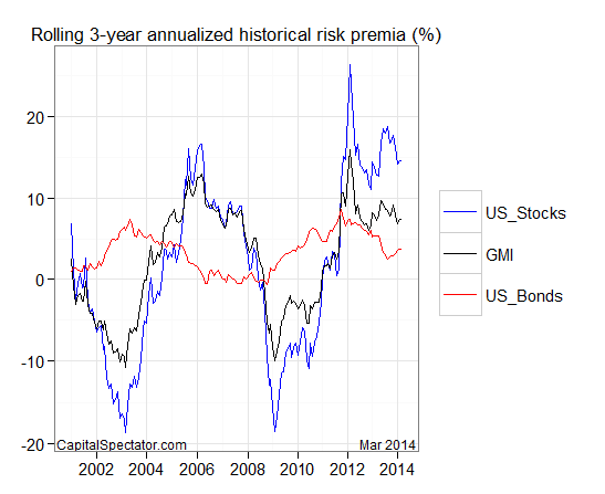
Note that GMI’s estimate is calculated by summing the weighted projections for all the major asset classes. To put these estimates in perspective, let’s look in the rear-view mirror via the record for the trailing three-year annualized risk premia for GMI, along with US stocks (Russell 3000) and US Bonds (Barclays Aggregate):

Let’s recognize right away that all the estimates in the table above come with the standard caveats. That said, it’s interesting to note the reduced outlook for GMI’s risk premium relative to recent history: 4.1% vs. 7.5% for the trailing three years through March 2014. That’s not surprising, given the relatively strong performance we’ve seen in recent years for risky assets—a bull run that’s probably due to moderate for the foreseeable future.

One way to use this data is to decide if GMI’s expected 4.5% risk premia will suffice. If we’re looking for a higher expected return (aren’t we all?), we might consider holding above-market-weights in those assets with more attractive opportunities and/or minimizing if not eliminating those markets with low expected returns.

In the long run, the average investor must hold the market portfolio, which means that the average investor is destined to earn the market’s return. If you’re not satisfied with the prospect of earning an average return, then you need some confidence for rethinking Mr. Market’s asset allocation. Developing that confidence isn’t easy or riskless, but estimating equilibrium risk premiums is a productive way to start the crucial process of deciding what the future will deliver.