In the previous installment in this series of analyzing a globally diversified portfolio we reviewed the results after adding a momentum-based risk-management system. The test suggested that a tactical overlay can be productive… maybe, depending on the details. Let’s continue to investigate our sample portfolio by taking a closer look at the underlying factors that are driving risk and return.

The tool of choice today is principal component analysis (PCA), a statistical methodology for reviewing the systematic variations in the data—the asset returns, in this case. PCA results, like any one procedure for risk analysis, shouldn’t be taken as irrefutable truth. But as one piece of a multi-dimensional risk-analysis application, PCA is a powerful means for developing a deeper understanding of portfolio structure.

Once again we’ll deploy R to do the heavy lifting if the toy modeling below. If you’re curious about the analytical details, here’s the code to replicate the results. Meanwhile, we’ll continue to use the 11 funds for testing a global mix of assets, spanning US and foreign stocks, bonds, REITs and commodities. For the tickers and outline of the asset mix, see the table here, in Part III of this series.

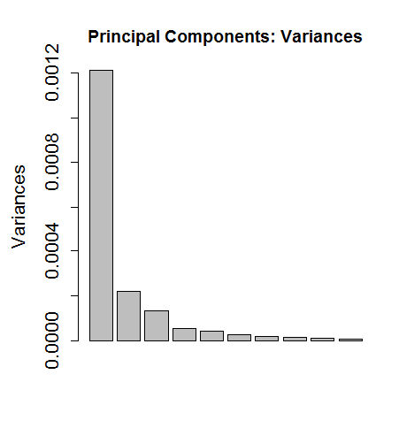
The first order of business is visually inspecting how the factors stack up. As the chart below shows, the first factor is the dominant source of risk in the portfolio. Looking at the details of the PCA output, however, tells us that the proportion of variance for factor 1 is around 38% of the total. The first five factors add up to around 75% of total portfolio variance and so these five factors probably explain most of what’s relevant.

Factor analysis covers a lot of terrain and so the details will be glossed over here. The general idea is that we’re looking for the key risk factors. Why? On a basic level it’s an issue of understanding what you own in terms of risk structure. A portfolio that’s dominated by one risk factor vs. a more diversified set of loadings is valuable information for a variety of reasons.

A quick example: if you discover that your strategy is reliant on, say, two factors, you can reduce the dimensionality of the data and focus on the critical sources of risk. In practical terms, this may lead you to reduce the number of funds/assets in the portfolio because it turns out that some of the holdings are redundant. Alternatively, if the analysis shows that five factors are at the core of the portfolio’s risk profile, you certainly want to include those factors in your analysis and emphasize techniques/funds that optimize the use of those five drivers.

One of several techniques for developing perspective on what’s relevant (and what’s not) in factor analysis is reviewing the correlations between asset returns and factors. As an example, here’s a summary of the correlations for the first five factors for each of the 11 funds in the sample portfolio:

           Dim.1        Dim.2       Dim.3       Dim.4       Dim.5
SPY    0.9445926 -0.136480111  0.10999994 -0.08898929  0.03229224
IJS    0.9043400 -0.198995669  0.13815051 -0.10967993 -0.03010719
EFA    0.9354801 -0.000726023  0.11533978  0.07653676 -0.03827676
EEM    0.9127910 -0.064754743  0.08385842  0.01376165  0.03219128
IEF   -0.3747603  0.686328014  0.44700312 -0.07727897  0.03126732
LQD    0.1397073  0.718997315  0.37054468 -0.22318364  0.41465711
VWEHX  0.3265305  0.519614178 -0.59462449 -0.33952736 -0.08871788
RPIBX  0.2026241  0.596555585  0.18910650  0.54249733 -0.49120014
PREMX  0.4915622  0.576742604 -0.41261496 -0.15494668 -0.12340411
QRAAX  0.4558299  0.161427682 -0.31876609  0.63031691  0.47897041
VGSIX  0.7981891 -0.153110300  0.25863832 -0.13643715 -0.09049941

A couple of quick observations. First, note that high degree of correlation between US equities (SPY) and the first factor (Dim.1): roughly 95%. By contrast, there’s a fair amount of negative correlation between the first factor and government bonds (IEF). If this was a real portfolio, we might investigate these conflicting relationships on a deeper level for additional insight on how to manage risk for the portfolio.

The main lesson in our simple example is that running a PCA analysis is often a valuable first step for profiling risk in a given portfolio. If you’ve carefully designed your strategy, there should be few if any surprises. Even if PCA doesn’t tell you anything you didn’t already know, it’s useful to have statistical confirmation of your assumptions.

Keep in mind that factor analysis comes in a variety of flavors and the PCA outline is just one facet. In a future post I’ll focus on another approach for factor analysis using regression analysis via the Fama-French factor set.

* * *

Previous articles in this series:

Portfolio Analysis in R: Part I | A 60/40 US Stock/Bond Portfolio
Portfolio Analysis in R: Part II | Analyzing A 60/40 Strategy
Portfolio Analysis in R: Part III | Adding A Global Strategy
Portfolio Analysis in R: Part IV | Enhancing A Global Strategy