Failure isn’t an option, but it happens. Modeling the possibility that a portfolio strategy will stumble isn’t exactly cheery work, but it’s a productive and necessary exercise for stress testing what the future can do to the best-laid plans for investing. The good news is that there’s a rainbow of options for estimating the potential for trouble. But it’s usually best to start with a basic framework before venturing into more exotic realms.

A solid way to begin is by calculating the probability that a portfolio’s return will fall short of a particular benchmark or return. Larry Swedroe, director of research for the BAM Alliance, last month wrote about the probability of underperformance from the perspective of four factor premiums. The technique is to assume a normal distribution of returns and model the outcome under a variety of scenarios. Normal distributions are problematic, of course, due to fat-tail risk. But as Swedroe correctly points out, a normal distribution is “reasonable for multi-annual returns data because annual returns data is approximately normally distributed for diversified portfolio.”

The details for the number crunching are straightforward. Several years ago The Calculating Investor outlined the procedure with an Excel spreadsheet. Let’s expand the concept a bit by applying the normal distribution function in R via the pnorm() command.

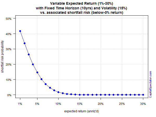
Assume we’ve designed a portfolio with a 10-year time horizon and expected annualized volatility (standard deviation) of 15%. Holding those variables constant, here’s the probability of generating a below-zero return over that span based on a range of expected returns for the portfolio:

Not surprisingly, the risk of suffering a negative result is substantial if we’re assuming a low return. A 1% annualized return carries a 40%-plus risk a sub-zero performance over a 10-year stretch. But as expected return rises, the risk of below-zero performance falls. As the portfolio’s projected return approaches 10%, the risk of losing money fades to a virtually nil possibility, given the assumptions about volatility and time horizon.

For another perspective, let’s vary the time horizon while holding the expected return and volatility constant by assuming the portfolio will earn 5% annualized with 15% standard deviation. As the next chart below shows, running the numbers through a normal distribution model tells us that the risk of sub-zero performance is considerable at a short time horizons. Starting at around 15 years, shortfall-return risk falls below a 10% probability. In other words, the longer the time horizon, the lower the probability of losing money.

Finally, let’s model various levels of expected volatility while holding constant the time horizon (10 years) and projected return (5%). The third chart below quantifies what intuition implies: higher portfolio volatility increases the probability of suffering a loss.

There are many variations on the simple examples above. For example, we can easily model the risk of falling short of the risk-free rate, an inflation-adjusted benchmark, or any other yardstick that’s considered relevant. We can also crunch the data by factoring in a fat-tails assumption for added reality. Ultimately, the goal is to design a modeling framework that’s customized for a specific portfolio.

The point is that a basic quantitative application is useful for deciding how a given portfolio might fare under extreme conditions. For instance, the procedure outlined above may reveal that a given set of assumptions is highly sensitive to small changes–a sensitivity that may not be obvious without a formal modeling effort. In that case, it may be time to go back to the drawing board for designing an asset allocation. After all, the price tag is always lower for discovering problems in the design stage as opposed to finding enlightenment when real money is at stake.

The future’s still uncertain, of course, but the first priority for the art/science of risk modeling is about minimizing the potential for surprises. Our capacity for insight is limited and so deploying diagnostic tests about what could happen fall well short of providing definitive clarity for the morrow. Estimating shortfall risk is no panacea, but it’s still useful. In fact, the only thing that’s worse than running this modeling procedure is not doing it at all.

* * *

Previous articles in this series:

Portfolio Analysis in R: Part I | A 60/40 US Stock/Bond Portfolio
Portfolio Analysis in R: Part II | Analyzing A 60/40 Strategy
Portfolio Analysis in R: Part III | Adding A Global Strategy
Portfolio Analysis in R: Part IV | Enhancing A Global Strategy
Portfolio Analysis in R: Part V | Risk Analysis Via Factors
Portfolio Analysis in R: Part VI | Risk-Contribution Analysis

Tail-Risk Analysis In R: Part I
Managing Portfolio Risk With Tactical Asset Allocation

Tactical Asset Allocation For The Real World