Making informed choices about active managers has never been anyone’s idea of a picnic, but ongoing developments in R packages eases the burden. Consider the essential work of factor analysis, which is a statistical technique for identifying the sources of risk and return in a portfolio through an objective prism. If nothing else, performing this task is the antidote to marketing hype that permeates the world of investment management. The gold standard for analyzing equity portfolios is regressing the returns against the Fama-French data set (FF), which is updated regularly at Professor Ken French’s web site. In the old days, the chore of downloading FF data, copying it into Excel, and running the analysis was quite tedious and time consuming, as this 2001 how-to article by Bill Bernstein reminds. If you had a deft hand in spreadsheet analysis, maybe you could slice and dice a fund’s history in ten minutes. Fast forward 13 years and you’ll find that factor analysis has become a snap. Using the R code I’ve written below, we can download the necessary data and run the analysis in less than ten seconds for each fund.
As a quick example, let’s analyze a fund using data for the ten years through June 2014 (the last month currently available on the FF site). Using Morningstar’s basic screening tool, I’ve chosen a top-performing five-star US equity fund with a strong trailing 10-year return: Lord Abbett Developing Growth (LADYX). Morningstar labels the fund as a small-growth portfolio. Let’s see how the numbers stack up when we run the returns through a factor-analysis framework in R (see code below to replicate the analysis).
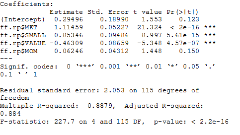
Here’s the output for LADYX:
As you can see under the Coefficients Estimate column on the left, which effectively lists the fund’s betas, LADYX has a bit of above-market risk relative to the stock market overall, as indicated by the 1.11 reading for the fund at the ff.rp.$MKT row. A 1.0 value for the ff.rp$MKT factor implies an equivalent degree of risk with stocks generally. Note that the fund’s high small-cap beta reading shows up at roughly 0.85. Clearly there’s a lot of traction with small stocks and so it’s obvious that small stocks are a key part of this fund’s risk tilt.
Meantime, note that the value reading is negative and the momentum beta is close to zero, which suggests that these factors aren’t relevant for the fund. Also, note the high Intercept value, which measures the fund’s alpha (returns above the benchmark). The positive 0.29% alpha contribution (roughly 3.5% a year) suggests that this fund is adding a fair amount of value over what an equivalent index fund exposed to these betas would deliver. No wonder, then, that Morningstar gave it a high five-star rating.
To play devil’s advocate, we might question how much value in LADYX’s results is really due to skill vs. luck based on the p-value for the Intercept reading. The p-value of 0.123 for the Intercept row (far right) tells us that the alpha reading isn’t statistically significant and so it may be due to noise. By contrast, the p-values for the MKT, SMALL, and VALUE readings are statistically significant. At the very least, the elevated p-value reading for the Intercept/alpha data tells us to take a deeper look at the fund before deciding that active-management talent reigns supreme here. (Generally, p-values below 0.05 suggest that we can reject the null hypothesis, which in this case is the default assumption that the performance results are due to random results. But discovering that the p-value is well above 0.05 for the alpha leaves room for doubt for thinking that stock-picking skill is a key factor here. Perhaps there’s genuine alpha, but the p-value at the very least implies that the market-beating results aren’t as high as the raw data shows.)
Keep in mind that the FF data set offers a range of nuance that allows us to run a variety of factor-analysis tests beyond the basic one shown above. The larger point is that the flexibility of R offers a rich toolbox for high-level analysis in the crucial business of measuring and evaluating sources of risk and return. Factor analysis alone isn’t the last word when it comes to fund analysis, but it’s surely a crucial part of any serious review. The fact that it’s easy to do in R only sweetens the deal.
R code to run factor analysis:
# load packages
library(tseries)

library(Quandl)

library(quantmod)
# download and process Fama-French factors
ff.a <- Quandl("KFRENCH/FACTORS_M")

ff.3 <- as.xts(ff.a[,-1],order.by=ff.a[,1])
ff.mom.a <- Quandl("KFRENCH/MOMENTUM_M")

ff.mom <- as.xts(ff.mom.a[,-1],order.by=ff.mom.a[,1])

ff.4 <-cbind(ff.3,ff.mom)
colnames(ff.4) <-c("MKT","SMALL","VALUE","RF","MOM") # add momentum factor
rf <-ff.4$RF # create separate risk-free rate vector
s.date <-"2004-06-30" # create start date for analysis
# create function to download and process mutual fund data

# to create monthly risk premium vector for mutual fund

f.data <-function(x,y) { # x=fund ticker; y=is risk-free rate via Fama-French data set

a <-get.hist.quote(instrument=x,start=s.date,quote="AdjClose")

b <-to.monthly(a,indexAt="lastof",OHLC=FALSE,drop.time=TRUE)

c <-na.omit(ROC(b,1,"discrete"))*100

d <-as.xts(head(c,-2)) # trim mutual fund return series set to match FF data set

e <-length(d)

f <-d-(tail(y,e)) # trim Fama-French risk-free data set to match trimmed mutual fund data

}
z <-f.data("ladyx",rf) # generate factor analysis data

len <-length(z) # Determine length of fund data set to match length of Fama-French data set

ff.rp <-tail(ff.4,len) # Trim Fama-French data set to match starting date as per s.date
factor.test.1 <-lm(z~ff.rp$MKT+ff.rp$SMALL+ff.rp$VALUE+ff.rp$MOM) # run regression analysis

summary(factor.test.1) # print factor analysis results

Pingback: The Whole Street’s Daily Wrap for 8/19/2014 | The Whole Street