Earlier this month I briefly reviewed a recent BlackRock report that highlighted that macroeconomic factors are typically driving investment strategy results. As a follow-up, let’s take a quick look at a basic real-world example of analyzing portfolios through a macroeconomic lens.

First, let’s recap why macroeconomic analytics are useful. The basic takeaway: macro influences (economic growth, inflation, real interest rates, etc.) are usually critical drivers of risk and return. Even if you’re not specifically targeting macro factors, portfolio results can often be traced to these forces. In turn, monitoring how macro exposures evolve in a portfolio deserves to be a key part of your routine risk-management analytics.

Depending on the portfolio, of course, the macro profile may already be obvious. A large-cap US equity strategy, for instance, tends to be heavily exposed to the economic factor. But intuition becomes less useful (and perhaps even misleading) for customized strategies that use, say, a mix of ETFs that target various asset classes. In that case, the macroeconomic factor profile isn’t obvious and so it’s valuable and quite often essential to quantitatively evaluate the portfolio on a regular basis.

---

Learn To Use R For Portfolio Analysis
Quantitative Investment Portfolio Analytics In R:
An Introduction To R For Modeling Portfolio Risk and Return
By James Picerno

---

As an example, let’s run the analytics on an ETF where the outcome is already known. Even before we crunch the numbers on the SPDR S&P 500 (SPY), it’s a safe bet that the economic factor dominates. That’s par for the course with a broad portfolio of stocks. But for illustration, let’s run through the process.

The first step is selecting data sets to proxy for the factors we’re interested in analyzing. This can get complicated, depending on what you’re trying to do. Indeed, there are dozens if not hundreds of factors to consider. In the interest of brevity, let’s use a toy example with five factors (and their related data set):

• Economic (US Coincident Economic Activity Index)
• Credit spread (CE BofAML US High Yield Master II Option-Adjusted Spread)
• Inflation (Consumer Price Index) 
• Commodities prices (Global Price Index of All Commodities)
• Real interest rates (based on risk premium for iShares TIPS Bond ETF (TIP))

One methodology is to run a multi-factor regression on the portfolio (SPY) against the five factors listed above. For a sample period, let’s use monthly data since 2007 through last month (Sep. 2019). As expected, the economy factor is by far the biggest influence in SPY, as shown in the regression output below.

Coefficients:
                    Estimate Std. Error t value Pr(>|t|)    
(Intercept)        -0.002729   0.003505  -0.779 0.437534    
commodities         0.236576   0.080977   2.922 0.004041 ** 
economy             4.584058   1.255592   3.651 0.000364 ***
real yield         -0.486947   0.156804  -3.105 0.002286 ** 
inflation          -2.565742   1.149944  -2.231 0.027203 *  
high yield bonds    1.293862   0.108999  11.870  < 2e-16 ***
---
Signif. codes:  0 ‘***’ 0.001 ‘**’ 0.01 ‘*’ 0.05 ‘.’ 0.1 ‘ ’ 1

Residual standard error: 0.02813 on 145 degrees of freedom
Multiple R-squared:  0.5923,	Adjusted R-squared:  0.5782 
F-statistic: 42.12 on 5 and 145 DF,  p-value: < 2.2e-16

Although the economic influence is the leading factor for SPY, note that high-yield bonds resonate too. Meanwhile, the inflation beta is deeply negative, suggesting the stocks tend to act negatively (positively) to high (low) inflation.

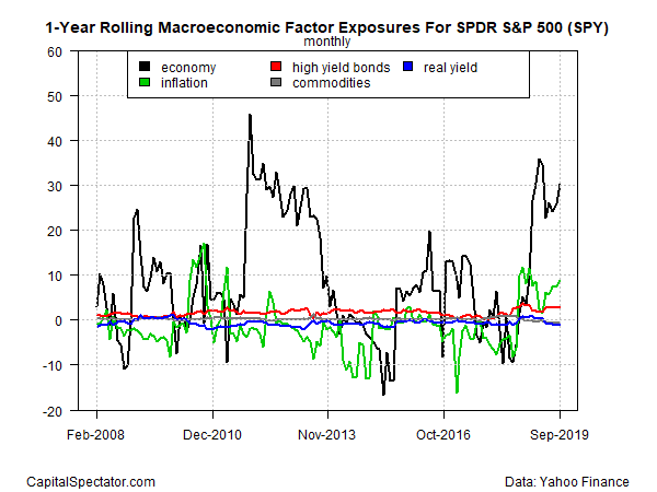
For another perspective, let’s graph how the various factors stack up on a rolling 12-month basis. In the chart below, it’s clear that the factor influences vary in the short term, although most of the time the economy beta is running the show (black line).

It’s also no surprise to find that different ETFs register different results. For instance, let’s run the same macro factor analysis from above on iShares Core US Aggregate Bond (AGG), a proxy for a broad mix of investment-grade fixed-income securities. As AGG’s regression results below show, the dominant influence now shifts to the real yield, which was basically insignificant for the SPY analysis. Note, too, that the inflation beta is negative for bonds, which is to say that high inflation will take a toll on nominal fixed-income portfolios such as AGG.

Coefficients:
                    Estimate Std. Error t value Pr(>|t|)    
(Intercept)         0.002431   0.000744   3.268  0.00135 ** 
commodities        -0.053677   0.017189  -3.123  0.00216 ** 
economy            -0.112860   0.266528  -0.423  0.67260    
real yield          0.494604   0.033285  14.860  < 2e-16 ***
inflation          -0.590173   0.244102  -2.418  0.01686 *  
`high yield bonds`  0.023622   0.023138   1.021  0.30898    
---
Signif. codes:  0 ‘***’ 0.001 ‘**’ 0.01 ‘*’ 0.05 ‘.’ 0.1 ‘ ’ 1

Residual standard error: 0.005971 on 145 degrees of freedom
Multiple R-squared:  0.6949,	Adjusted R-squared:  0.6844 
F-statistic: 66.06 on 5 and 145 DF,  p-value: < 2.2e-16

The value of looking at portfolios through a macro lens is that hidden risks may be revealed. That includes highlighting unintentional factor bets.

The good news: creating a diversified set of factor exposures (or an intentional focus on concentrating those bets) is straightforward, and it starts with analyzing the portfolio. By contrast, hoping for the best and risking unintentional bets is asking for trouble. 

---

Is Recession Risk Rising? Monitor the outlook with a subscription to:
The US Business Cycle Risk Report

---